Vignette 02 — Babbitt (Cu-Ni, Duluth Complex): feet, unassayed core, and estimating on dense data
Contents
- 1. Files that don't state their units
- 2. Validation, and a bug this data exposed
- 3. 61 % of the core was never assayed: unknown ≠ zero
- 4. Assay: populations, a top-cut that is justified, domains
- 5. Variogram and block model
- 6. Estimate
- 7. Cross-validation: where the third bug was found
- 8. Grade-tonnage and a plausibility check
- 9. This is not a Mineral Resource. What it would take:
- Try it yourself
- Attribution
Bahasa Indonesia: versi Bahasa Indonesia · Previous vignette: 01 — Thalanga
| Data | The Babbitt (Cu-Ni-PGE) drill database, Duluth Complex, Minnesota — from the Natural Resources Research Institute, University of Minnesota, Duluth Complex database (NRRI/TR-2003/21), as distributed with pygslib's Tutorial 1 (MIT). The data is not copied into this repository; the runner reads a local copy or downloads it from a pinned pygslib commit. |
| Modules | Core → Assay → Resource |
| Lessons | Units in feet · 61 % of the core never assayed · when a top-cut is right · estimating on dense data · why an "estimate" is not yet a "resource" |
| Reproducible | python3 docs/vignettes/tools/run_babbitt.py (about 130 s). Every number is read from ../data/babbitt.json and re-checked by test_vignettes.py. |
Vignette 01 (Thalanga) was a case of too little data: 13 holes with no lithology. Babbitt is the opposite: 399 holes, 35,616 assay intervals, more than 160 km of core. That much data sets different traps. Nothing looks wrong, the software runs smoothly, and the answer can still be off by an order of magnitude.
The Babbitt deposit (now known as Mesaba) is disseminated Cu-Ni-PGE mineralisation in the basal part of the Duluth Complex, a layered intrusion. The mineralisation is continuous, low-grade and broadly parallel to the gently dipping basal contact. Teck's public description gives a geological resource of more than 1 billion tonnes at about 0.43 % Cu and 0.09 % Ni. That is our plausibility benchmark in §8.
1. Files that don't state their units
collar_BABBITT.csv   BHID, XCOLLAR, YCOLLAR, ZCOLLAR           ← no depth column
survey_BABBITT.csv   BHID, AT, AZ, DIP
assay_BABBITT.csv    BHID, FROM, TO, CU, NI, S, FE             ← no units in the header
Nothing says that every length in these files is in feet. You have to find the clues yourself:
- the dominant sample length is exactly 10.0 (78 % of intervals), a round feet number (10 ft = 3.048 m);
- collar elevations are about 1,590, while the ground in north-east Minnesota is about 480 m above sea level. The number only makes sense in feet;
- the collars spread over 18,006 × 11,316. As metres that is 18 × 11 km, far too wide for one deposit.
Read as metres, every length is 3.28 times too long, so every volume is 3.28³ = 35.3 times too large, and so are the tonnes and the metal. There is no error and no warning, because a feet file is not "broken".
In Core: Upload → Import Options → Length unit in the files: Feet (convert to metres), then upload the three files. Core multiplies collar X/Y/Z, survey depth and from/to by 0.3048, and states it in the import report and in every export's header:
# lengths: metres (converted from feet x0.3048 on import: collar x/y/z/depth, survey depth, from/to)
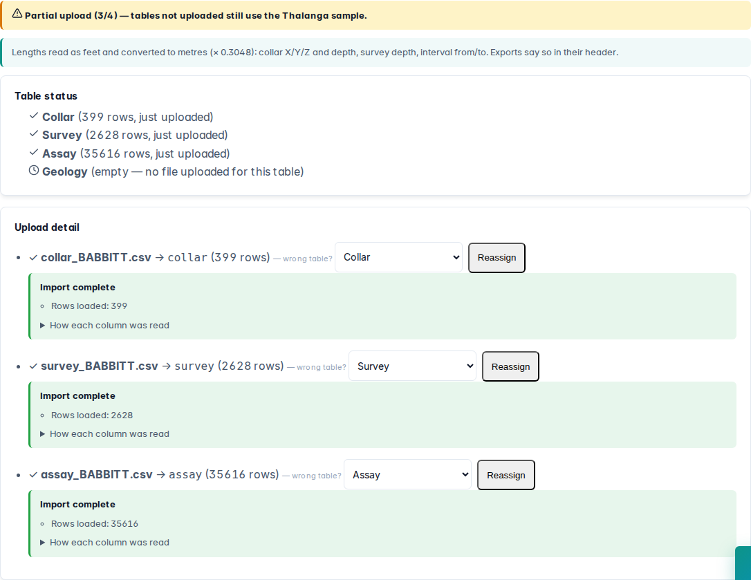
The result is a 5,488 × 3,449 m footprint, which is plausible for one deposit.
This option was added to GeoSuite because of this vignette. Before it, there was no way to import feet data correctly.
2. Validation, and a bug this data exposed
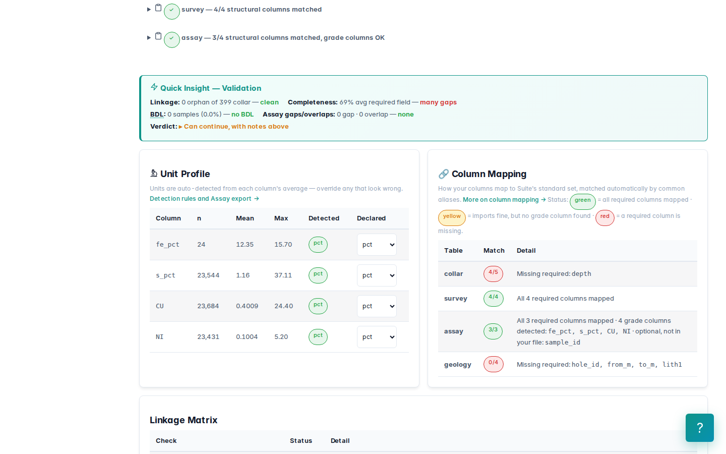
The table links are clean: no orphan holes, no duplicate collars, no gaps or overlaps. Two notes:
- No end-of-hole depth on the collars. The collar completeness check fails (80 %) because there is no
depthcolumn. Core now extends each trace to the deepest logged interval. - Two holes have a single survey station (at depth 0).
Together, these two exposed a real bug in GeoSuite. A trace used to be extended only to collar.depth. Without that column, every sample below the last survey station was stacked on that station. On a single-station hole, every sample sat on the collar: 97 samples in Babbitt. Take B1-001 (−60° towards 327°): the mid-point of its deepest interval (about 129 m along the hole) belongs at elevation 382.53 m, not at the collar's 494.05 m. The 382.53 m figure is recomputed with trigonometry in the runner and matched against Core's export.
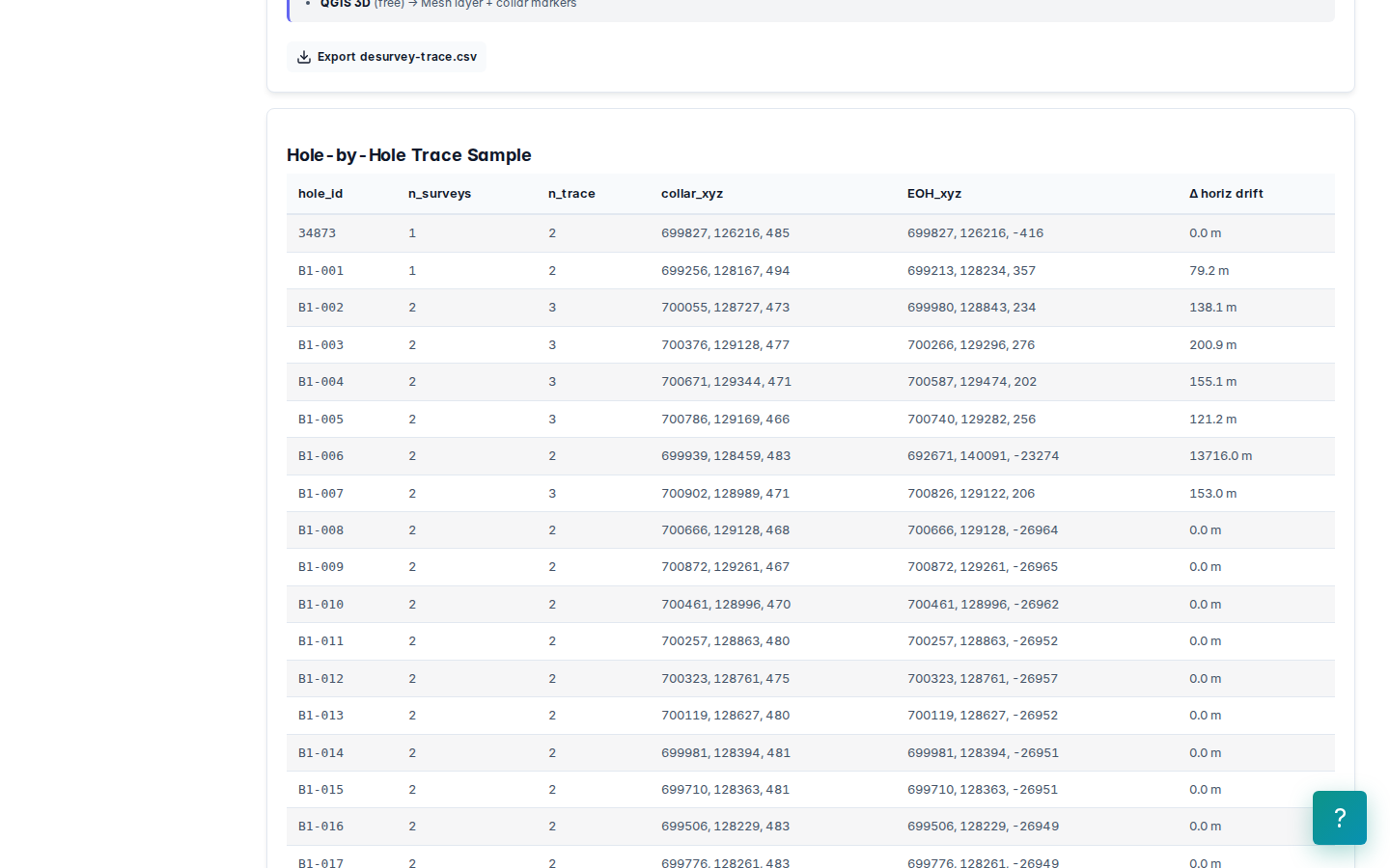
The bug is fixed and now guarded by test_lab_conventions.py. The lesson for geologists: "no error" is not "the samples are in the right place". Check one or two holes by hand. It is cheap, and it can save the whole model.
3. 61 % of the core was never assayed: unknown ≠ zero
| Length | |
|---|---|
| Total drilled | 164,967 m |
| Assayed (Cu present) | 63,726 m |
| Never assayed | 101,241 m (61.4 %) |
Take hole 34873: 0–766.6 m is unassayed, a run of cover rock above the basal zone. Length-weighted mean Cu:
| Treatment of unassayed intervals | Mean Cu |
|---|---|
| Unknown (left out of the mean) | 0.3638 % |
| Zero ("barren for sure") | 0.1405 % |
That is a factor of 2.6, and even a well-known geostatistics tutorial takes the "zero" route. Which is right? It depends on the geology, and that decision belongs to the geologist, not the software:
- cover intervals (rock above the intrusion, sediments) that were left unassayed because they are obviously barren → zero can be justified, outside the mineralised domain;
- intervals inside the zone that were skipped to save assay budget → zero is a serious low bias.
GeoSuite treats unassayed intervals as unknown: the composite grade is blank, not zero. Since this vignette, composite coverage counts only length that was actually assayed. Composites inside unassayed core used to report coverage 1.0 with blank grades. Now 33,236 composites honestly report being less than 50 % informed.
4. Assay: populations, a top-cut that is justified, domains
Upload Core's master CSV to Assay. The unit-less CU, NI, S, FE columns are read as percent (cu_pct …). The values (median Cu 0.30) fit percent, not ppm. Check it yourself: 0.30 ppm Cu makes no sense in a sulphide zone.
Cu–Ni correlation is r = 0.711, with a median Ni/Cu ratio of 0.241. That is the typical Duluth magmatic-sulphide signature: about four times more Cu than Ni, and the two move together.
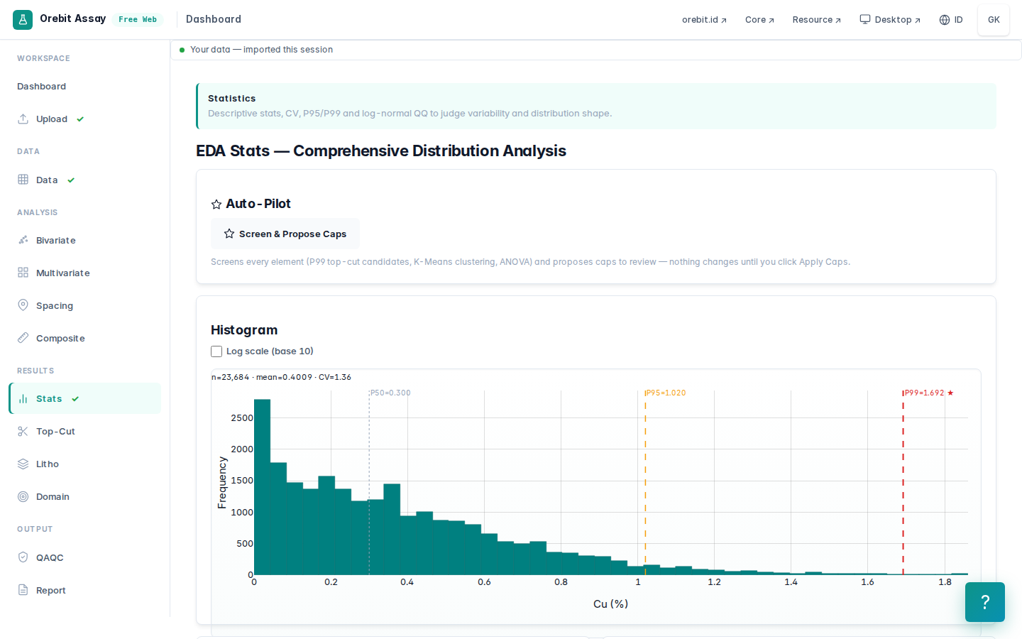
The distribution
| Cu (%) | |
|---|---|
| Median / P99 / P99.9 | 0.30 / 1.70 / 6.5 |
| Maximum | 24.4 |
Above about 5 % sit a few dozen semi-massive sulphide samples: 5–24 % Cu with up to 18 % S. They are real, but they form a thin, discontinuous population inside 0.3–1 % disseminated mineralisation.
Top-cut diagnostics: the app declines to propose a number
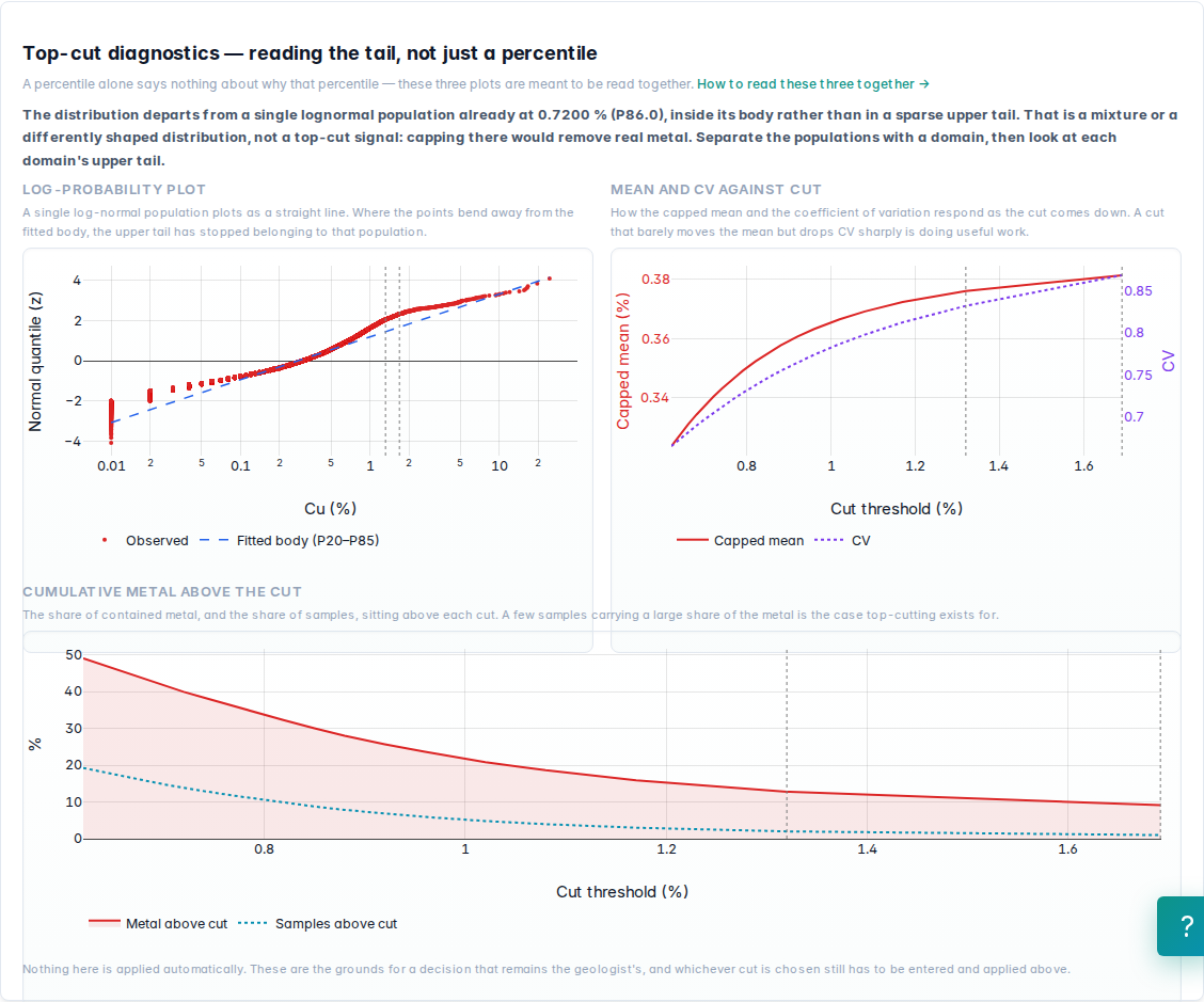
The Cu distribution departs from a single lognormal population from 0.72 % (P86) onwards, inside its body rather than in a sparse upper tail. An earlier GeoSuite version offered that point as a "disintegration candidate". Capping at 0.72 % would have removed 15 % of the metal. The app now calls it what it is: a population mixture, fixed by domaining, not by a top-cut.
Decision: domain first, then a 3 % Cu top-cut
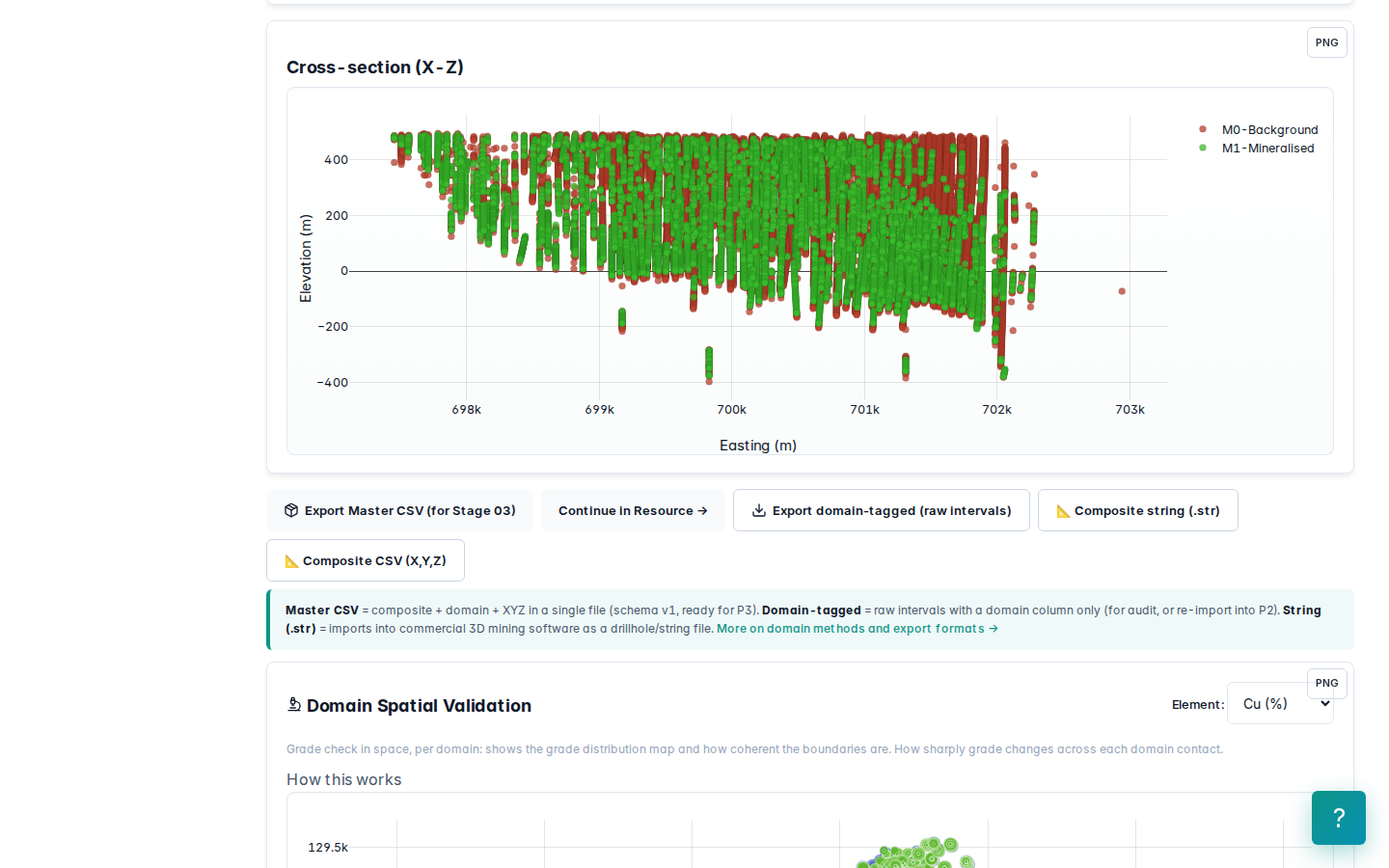
- Domain: a 0.2 % Cu grade shell. It holds 91.4 % of the metal in 62.5 % of the assayed length. The 0.2 % boundary sits near the lower edge of Duluth disseminated mineralisation and separates almost barren intrusive rock.
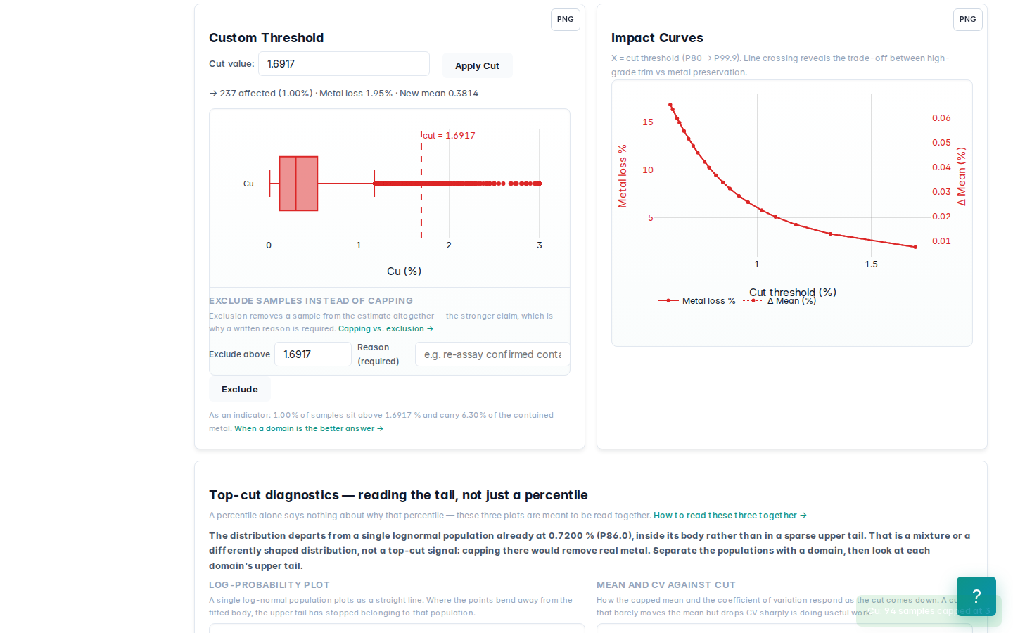
- Top-cut at 3 % Cu, applied to the raw assays before compositing:
| Assays capped | 94 |
| Metal removed, length-weighted (app = independent calculation) | 1.68 % |
| CV inside the 0.2 % shell: before → after | 1.07 → 0.66 |
| P99.5 inside the shell | 3.5 |
Why a top-cut is right here when it was wrong at Thalanga (vignette 01):
| Thalanga | Babbitt | |
|---|---|---|
| High grades come from | the main ore population (massive sulphide) | thin, sparse semi-massive segregations |
| Continuity between holes | the mined lens | none: one or two samples per hole |
| Search reach vs population size | small radius, large population | 200 m radius, metre-scale population |
| CV inside the domain | 1.15 | 1.07, down to 0.66 by capping 94 samples |
One 24 % Cu assay with a 200 m search spreads massive-sulphide grade into dozens of blocks that are really disseminated. That is what the top-cut prevents. The better geological alternative would be a separate high-grade domain, but without lithology logging it cannot be built.
The export header records the decision:
# topcut: cu_pct cut=3.0000 affected=94/23684 metal_removed=1.68% (length-weighted) applied_by=manual
Earlier versions summed assay values without length weighting and reported 2.99 %. Metal is grade × length, so a 0.2 m sample must not weigh the same as a 3 m interval. Now fixed, and checked against the independent calculation by
test_vignettes.py.
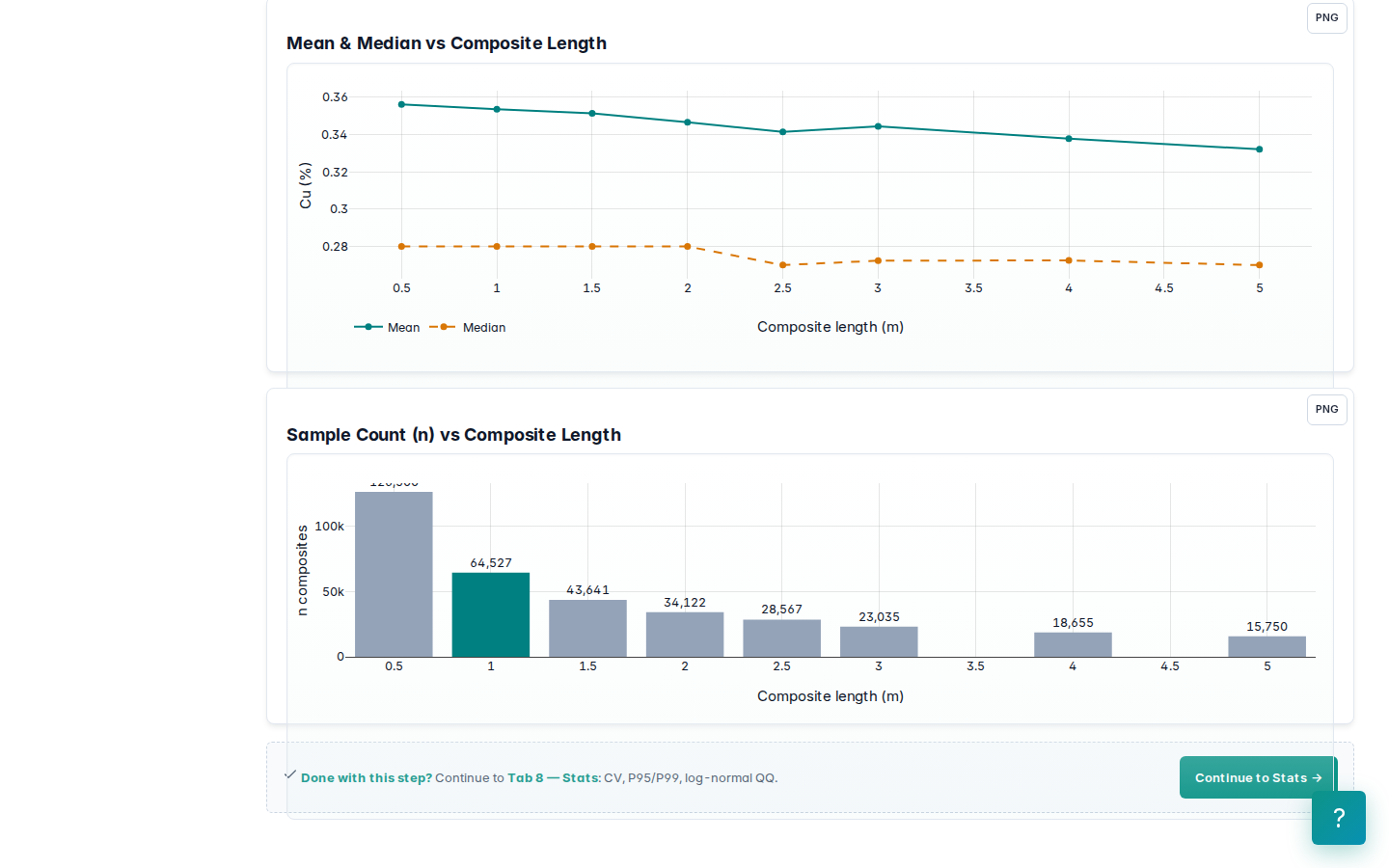
10 ft (3.048 m) compositing
| Composites | 55,119 (M1: 13,464, M0: 41,655) |
| M1 composites: mean / CV / max. | 0.5235 % / 0.59 / 3.0 % |
| M1 footprint (X × Y × Z) | 4,824 × 3,453 × 869 m |
The second bug this stage exposed was in composite coordinates. Each composite used to be given the mid-point of the raw interval that contained it. Every composite cut from one long interval, such as the 252 composites from the 766 m interval in hole 34873, landed on one and the same point. Zero-distance pairs with different grades inflate the nugget, and duplicate points make the kriging system singular. Positions are now interpolated along the hole at each composite's own mid-depth (test_estimation_inputs.py).
5. Variogram and block model
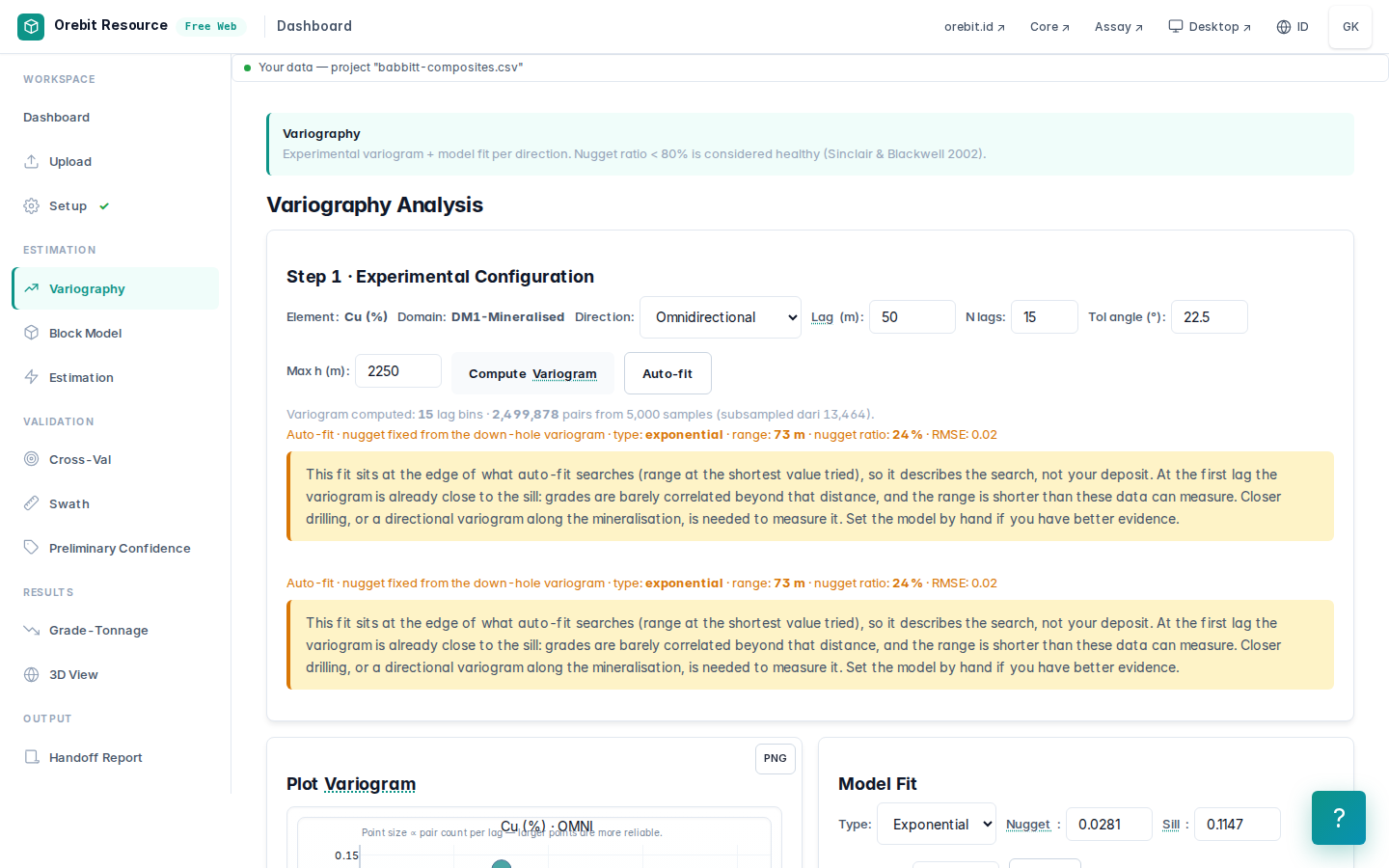
Nugget from the holes. Compute the Variogram Downhole first (Variography tab, 2 m lags): 183,031 pairs of samples within the same hole. Most samples are 10 ft (3.05 m) long, so adjacent samples pair up at 3 m, where γ is 0.035 (%²). The 1 m bin, from a few shorter samples, gives 0.028; the app takes the lowest of the first three lags. Either way the nugget is a quarter to a third of the sill.
Then between holes. Auto-fit holds the nugget at the down-hole value: exponential, nugget 0.028, sill 0.115 (%²), about 24 % nugget. Range 72.5 m, and the app flags it as the shortest range the fit tries. In the first lag (0–50 m, down-hole and between-hole pairs pooled), γ is already 0.093, 98 % of the data variance.
Earlier revisions of this vignette reported "nugget 0.063 = 60 %". Like on Thalanga (vignette 01 §7), that was the ceiling of the fitting grid, not the deposit. See the down-hole variogram for the real short-range structure.
Nearest between-hole spacing: median 107 m, P90 150 m. The variogram range is shorter than the hole spacing. The measured spatial structure comes almost entirely from down-hole pairs. At hole spacing, kriging has almost no correlation to work with and will return something close to a local mean. In a layered deposit like this one, the honest variogram is a directional variogram parallel to the layering. We record that as a limitation.
Block size: the app suggests 55 × 55 × 28 m. Used: 50 × 50 × 15 m (about ½ the hole spacing; 15 m ≈ 50 ft, an open-pit bench height), giving 237,475 blocks.
6. Estimate
Search 200 × 200 × 30 m (horizontal, about twice the hole spacing; vertically tight because the mineralisation is layered), 4 to 16 composites. Two runs: without and with the domain boundary (Keep blocks inside the domain, see vignette 01 §8: a block joins the domain only if its nearest composite, of any domain, is in it).
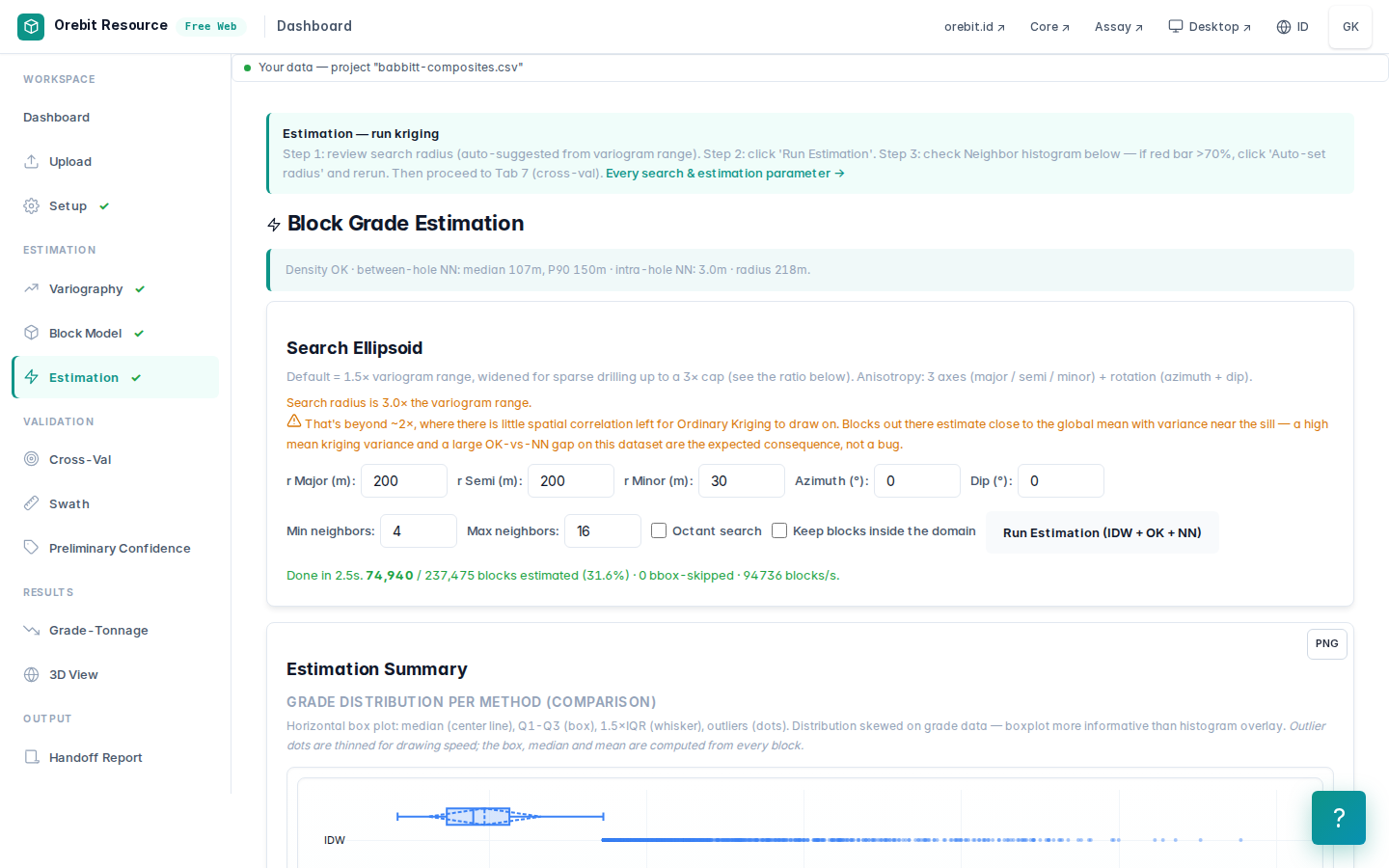
| No domain boundary | With domain boundary | |
|---|---|---|
| Blocks estimated | 74,940 | 26,842 |
| Blocks within reach removed by the boundary | — | 209,506 |
| Mean Cu grade (OK) | 0.474 % | 0.503 % |
| Tonnes (2.8 t/m³) | 7,869 Mt | 2,818 Mt |
| Cu metal | 37.3 Mt | 14.2 Mt |
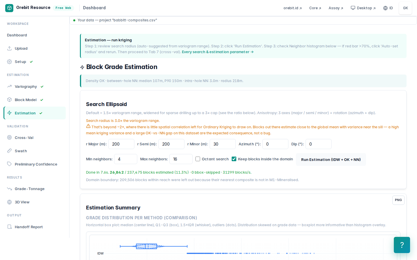
On dense data the boundary removes almost two-thirds of the tonnage: blocks within 200 m of a ≥ 0.2 % Cu composite whose nearest composite is < 0.2 % Cu rock or unassayed core. The mean grade rises because those "diluted" edge blocks leave.
Note a hidden decision: Assay labels unassayed composites M0, so 33,236 composites of unassayed core act as boundary too. For cover rock above the intrusion that is right. For intervals inside the zone that were skipped by the assay budget, it can cut out ore. That is a geologist's decision and must be written down (§3).
Global mean check (with the boundary): OK 0.503 % and NN 0.509 %, 1.1 % apart. Tonnage recheck: 26,842 blocks × 37,500 m³ × 2.8 t/m³ = 2,818 Mt. It matches.
7. Cross-validation: where the third bug was found
The earlier leave-one-out searched for neighbours only among the 200 random samples being tested, not among the 13,464 composites. On dense data each test sample "saw" a few random points kilometres away, so only 10 of 200 could be computed. The random sample was also unseeded, so the numbers changed on every run. Neighbours now come from all samples, and the subsample uses a fixed seed.
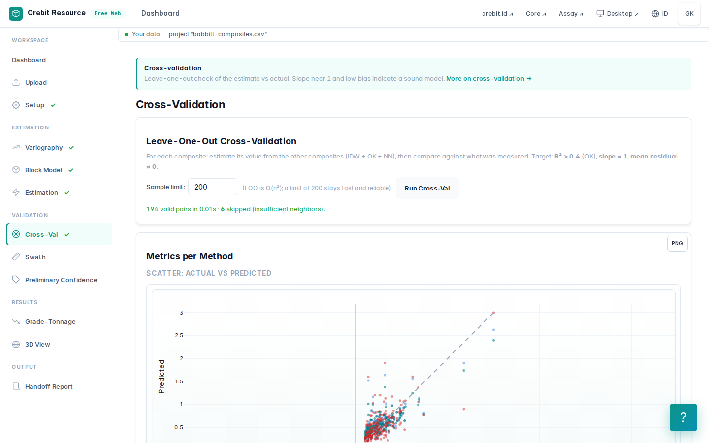
| n = 194 of 200 | OK | IDW | NN |
|---|---|---|---|
| Slope (estimate on actual) | 0.62 | 0.68 | 0.68 |
| r² | 0.67 | 0.62 | 0.47 |
| Mean bias | +0.02 | +0.03 | +0.02 |
The estimate is globally unbiased, but a slope of 0.62 means substantial smoothing: high grades are strongly under-estimated and low grades over-estimated. That is what a range shorter than the hole spacing produces (§5). With the old grid-ceiling nugget of 60 % the slope was 0.50; reading the nugget from the holes improved it, but no variogram can make up for drill spacing. On the grade-tonnage curve this means too many tonnes at low cut-offs and too low a grade at high cut-offs. The curve must not be used to choose a mining cut-off without a change-of-support correction.
8. Grade-tonnage and a plausibility check
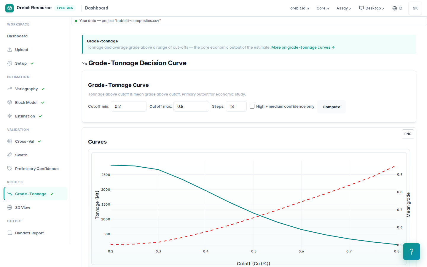
| Cu cut-off | Tonnes (Mt) | Cu grade |
|---|---|---|
| 0.2 % | 2,818 | 0.503 % |
| 0.3 % | 2,671 | 0.516 % |
| 0.4 % | 1,960 | 0.575 % |
| 0.5 % | 1,203 | 0.655 % |
| 0.6 % | 656 | 0.745 % |
| 0.8 % | 150 | 0.952 % |
Against the public description (> 1 billion tonnes @ ~0.43 % Cu), the grade is comparable. Without the domain boundary our tonnage was about 8 times larger; with it, still about 2.8 times. The remaining gap is not units (feet were converted) and no longer extrapolation into wall rock. It is the reporting principle most often forgotten:
A Mineral Resource must have reasonable prospects for eventual economic extraction (RPEEE). Our estimate is a geological inventory: every block inside the 0.2 % Cu domain, down to 869 m below surface. A reported resource is bounded by:
- an economic cut-off (for Cu-Ni-PGE usually an NSR value, not Cu alone). A 0.4 % Cu cut-off alone already brings the tonnage down to 1,960 Mt;
- an optimised pit shell, so deep blocks below the pit floor are not counted;
- sensible confidence classification, so blocks far from data are left out.
Density adds to this: 2.8 t/m³ is an assumption. Duluth troctolite/gabbro typically runs about 2.9–3.0 t/m³, and measured density would add tonnes.
9. This is not a Mineral Resource. What it would take:
- [ ] Lithology logging and a geological model of the basal zone, cover rocks and semi-massive sulphide;
- [ ] A directional variogram parallel to the layering, and a search ellipsoid that follows its dip;
- [ ] A high-grade domain for semi-massive sulphide instead of a top-cut;
- [ ] A geologist's decision on unassayed intervals inside the zone;
- [ ] Measured density; QA/QC for the historical and modern drilling campaigns;
- [ ] Cu-Ni-Co-PGE NSR, a pit shell and an economic cut-off (RPEEE);
- [ ] A change-of-support correction before reading the grade-tonnage curve;
- [ ] Classification and reporting by a Competent / Qualified Person (KCMI 2017 / JORC 2012 / NI 43-101 / S-K 1300).
Try it yourself
- Re-import without switching on Feet and compare the tonnes with §6. The ratio should be about 35.
- Run without the top-cut. How many blocks above 1 % appear, and where?
- Raise the domain cut-off to 0.3 %. How do the nugget and the cross-validation slope change?
- Limit the horizontal radius to 110 m (about the hole spacing). How many tonnes disappear, and which blocks?
Attribution
Babbitt drill data: Natural Resources Research Institute, University of Minnesota Duluth — Duluth Complex drill-hole database (NRRI/TR-2003/21), distributed with pygslib (© Adrian Martinez Vargas, MIT licence) in doc/source/Tutorial_1/Babbitt. Mesaba resource description: Teck publication (CESL, ALTA 2009) on nickel recovery from Mesaba concentrate. For current official figures, see the Mesaba NI 43-101 technical report published by PolyMet Mining (2022).
Source of this page: docs/vignettes/en/02-babbitt-cuni.md · GPL-3.0 · github.com/ghoziankarami/geosuite