Vignette 01 — Thalanga (VMS Zn-Pb-Cu-Ag-Au): from raw public data to a resource screen you can defend
Contents
- 0. Geological context and an independent benchmark
- 1. Load the data (Core)
- 2. Laboratory grade codes: negative numbers are not numbers
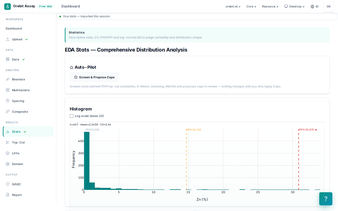
- 3. Validation: find, decide, record
- 4. Desurvey and crop to the deposit area
- 5. Know the populations before deciding anything
- 6. Assay: choose the commodity, test the top-cut, build the domain
- 7. Resource: setup, variogram, block model
- 8. Estimation: the most important lesson in this vignette
- 9. Cross-validation
- 10. Confidence screen and grade-tonnage
- 11. Density: one number that moves tonnage by ±30 %
- 12. Sanity check against historical production
- 13. This is not a Mineral Resource. What it would take:
- Try it yourself
- Reproducing this vignette
- Attribution
Bahasa Indonesia: versi Bahasa Indonesia
| Data | NEQ Deposit Atlas – Thalanga (ds100103), Geological Survey of Queensland, CC BY 4.0 — https://geoscience.data.qld.gov.au/dataset/ds100103. It is also Orebit Core's built-in sample, so you can follow along without downloading anything. |
| Modules | Core → Assay → Resource |
| Time | about 45 minutes by hand |
| Outcome | An honest grade-tonnage screen, with the list of reasons it is not yet a Mineral Resource |
| Reproducible | node build/build.mjs && python3 docs/vignettes/tools/run_thalanga.py. Every number on this page is read from ../data/thalanga.json, which that script writes. test_vignettes.py fails the build if the app starts producing different numbers. |
This vignette deliberately avoids "clean" synthetic data. A government compilation like this one is what exploration geologists actually receive: hundreds of holes from many companies over many decades, laboratory codes that changed over time, shallow geochemical holes mixed with deep diamond holes. The aim is not a pretty number. The aim is to show every decision a geologist must make, why, and what happens if it is skipped.
0. Geological context and an independent benchmark
Thalanga is a volcanogenic massive sulphide (VMS) Zn-Pb-Cu-Ag-Au deposit in the Mount Windsor Subprovince, about 65 km south-west of Charters Towers, Queensland. The underground mine operated from 1989 to 1998 and produced 4.7 Mt @ 8.3 % Zn, 2.6 % Pb, 1.9 % Cu (mining-technology.com).
That production figure is our benchmark. Never judge an estimate by "the program finished without errors". Ask instead: is the answer plausible against something known independently? At the end (§12) we compare the screen against this benchmark and explain the difference.
One honest note up front: the dataset has no lithology logging for the deposit's diamond holes. No lithology means no geological model. That limits everything downstream, and you will see the consequences clearly.
1. Load the data (Core)
Open Orebit Core. The Thalanga dataset loads automatically as the sample.
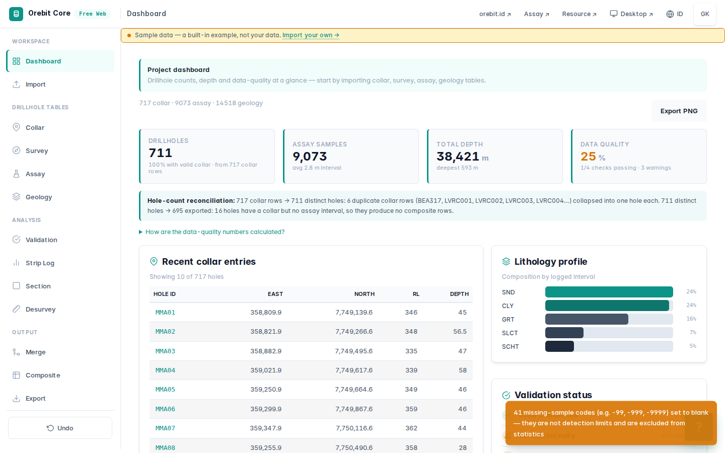
| Table | Rows |
|---|---|
| Collar | 717 |
| Survey | 667 |
| Assay | 9,073 |
| Geology | 14,518 |
Before you look at a map, look at the hole types:
| Drill type | Holes |
|---|---|
| BEDRK (shallow bedrock geochemistry) | 520 |
| REVC (RC) | 55 |
| PERC (percussion) | 45 |
| RAB | 39 |
| ACORE | 21 |
| TCH (trench) | 19 |
| DD (diamond) | 18 |
Lesson one: this is a regional compilation, not a deposit drill database. Three-quarters of the holes are shallow geochemical holes drilled to find anomalies, not to measure tonnes. Mix them all into an estimate and hundreds of "background" samples from tens of kilometres away drive the statistics and the variogram. That is why the crop step (§4) exists.
2. Laboratory grade codes: negative numbers are not numbers
Legacy assay data uses negative numbers as codes, and their meaning differs between labs and decades. Core detects them on import and applies one documented rule (src/shared/io/grades.js):
- ordinary negative values (−0.01, −5, −0.0001) → below detection, used as half the detection limit;
- all-nines codes (−999, −9999 …) or a negative value whose magnitude exceeds the column's largest positive value → missing (blank). No detection limit can be higher than the highest grade ever measured;
>X(over-range) → X, flagged.
On Thalanga: 2,428 below-detection values and 41 missing codes.
| Column | < detection | Missing codes | Max. positive value |
|---|---|---|---|
| au_gpt | 1,223 | 0 | 1,380 |
| ag_gpt | 578 | 19 | 9,560 |
| s_pct | 485 | 7 | 5 |
| cu_ppm | 68 | 0 | 114,200 |
| pb_ppm | 68 | 15 | 248,000 |
| zn_ppm | 6 | 0 | 406,000 |
Why this matters: the Pb column contains the code −995,000 and Ag contains −9,910,000. Software that treats every negative as "half detection" hands those samples 49 % Pb and 4,955 g/t Ag, which is 15 fake bonanzas. Software that treats them as zero, or silently drops them, lowers the mean without a trace. The column-maximum rule separates the two cases without per-lab guesswork, and the 1,223 Au detection-limit values from several eras (−0.01, −0.05, −0.0001) are still correctly handled as real low values.
Check it yourself: on Core's Validation tab the row Below-detection (negative) grade values reads 0 after import. That does not mean the data was clean. It means every code was translated and logged.
3. Validation: find, decide, record
Core's Validation tab runs 16 checks.
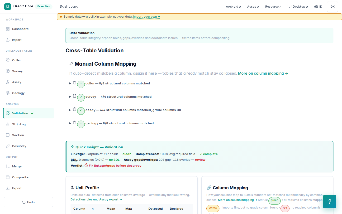
| Check | Before | After fixes |
|---|---|---|
| Collar without survey (assumed vertical) | 259 holes ⚠ | 259 ⚠ |
| Collar without assay | 16 holes ⚠ | 16 ⚠ |
| Collar without geology | 381 holes ⚠ | 381 ⚠ |
| Duplicate collar hole_id | 6 ✗ | 6 ✗ |
| Assay interval gaps | 208 ⚠ | 206 ⚠ |
| Assay interval overlaps | 115 ✗ | 113 ✗ |
| Linkage verdict | FIX REQUIRED | FIX REQUIRED |
What the findings actually are (checked row by row):
- 6 duplicate collars. LVRC001–LVRC005 appear twice, under two programmes (RGMWP and TCLV), 1–5 cm apart: the same holes compiled twice. BEA317 appears as both ACORE and BEDRK.
- 115 overlaps. Mostly re-samples or field composites compiled alongside the originals. Example: TCRC11 holds a 4–5 m interval and a 4–8 m composite.
- 259 holes without survey are assumed vertical. All of them are shallow (236 BEDRK, 20 percussion, 3 RC; median depth 36 m, deepest 150 m), so the effect is small. On deep holes that assumption is fatal (§4).
- 381 holes without geology, including every diamond hole in the deposit.
Two fixes, and why only two
- Two spot samples in TH37 (190.0–190.2 m and 490.0–490.2 m, sample IDs
TH37190,TH37490) sit entirely inside longer intervals of the same hole. They are check samples that were compiled in. Both are deleted; otherwise the same rock is counted twice. - Au 1,380 g/t in TH35 100.0–100.2 m. The next-highest value in the entire dataset is 1.69 g/t, about 800× lower. In the same interval Ag is 1 g/t and Zn 1,210 ppm. A gold bonanza with no silver and no base metals makes no geological sense in a VMS system; a unit or decimal error is far more likely. The value is blanked, not "corrected" to 1.38. We do not guess what the lab certificate says. Blank it, record it, request the original certificate.
Both edits are made in Core's data editor and are logged automatically in the CHANGE_LOG:
assay: 1 rows edited, 0 added, 2 deleted
The CHANGE_LOG travels with the export. Anyone who receives your file can see exactly what was changed and when.
Why the verdict stays "FIX REQUIRED", correctly
The remaining problems (LVRC/BEA duplicates, the hundreds of TCRC-type overlaps) are all in regional holes outside the deposit area. A senior geologist does not "clean" data they will not use just to turn the indicator green. That data is explicitly excluded by the area boundary (§4), and the reason is written down. A red verdict here is an honest record, not a failure.
4. Desurvey and crop to the deposit area
Desurvey
The Desurvey tab detects the dip convention from the data: positive_down, meaning positive dip points downward. Result: 711 holes desurveyed, 0 bad surveys.
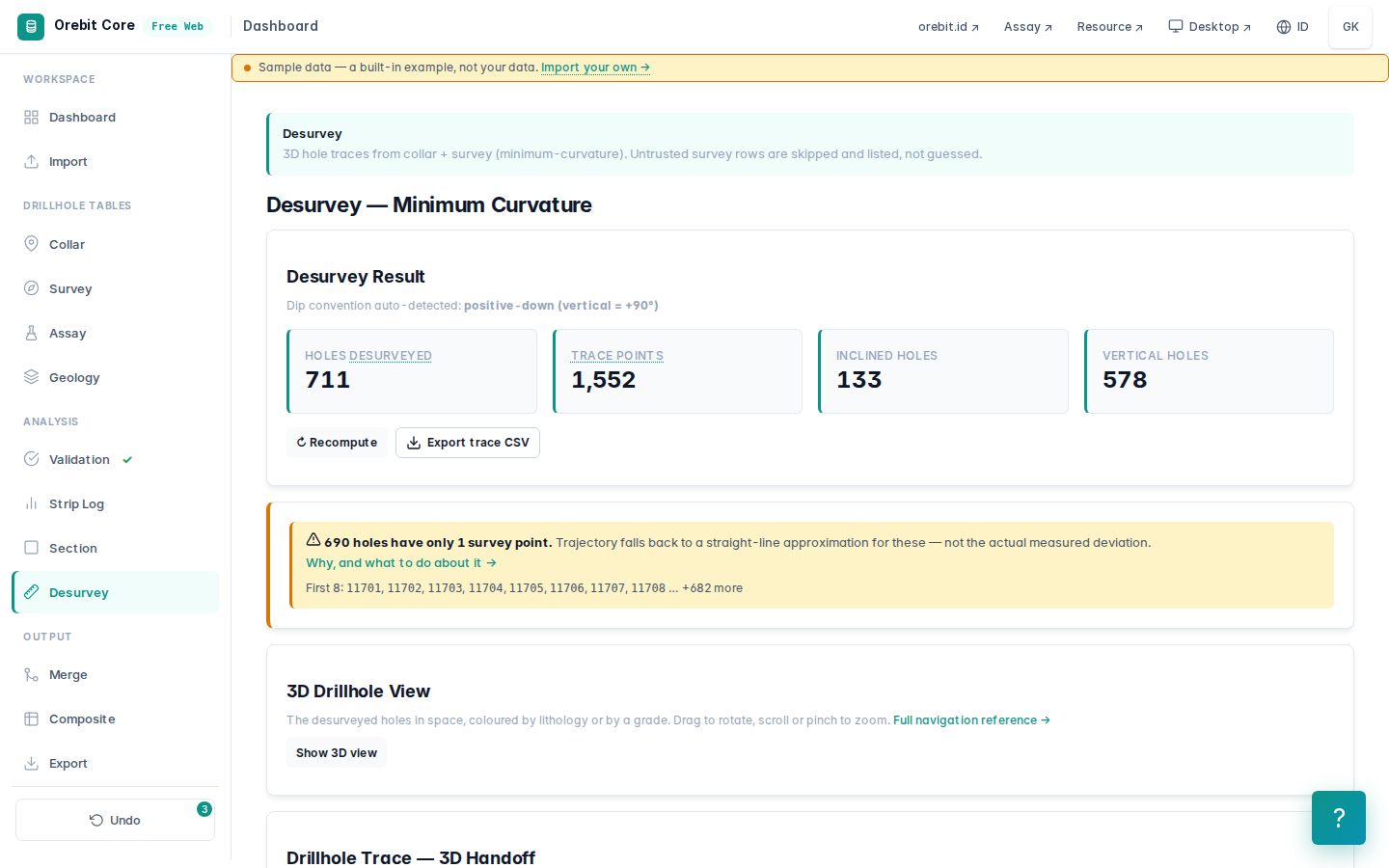
Thalanga's diamond holes flatten strongly towards the bottom:
| Hole | End depth | Elevation at end of hole (z) |
|---|---|---|
| TH1 | 257 m | 140.9 m |
| TH5 | 395.9 m | 117.2 m |
| TH40 | 593.3 m | −103.1 m |
TH5 is almost 400 m long but drops only about 180 m and finishes nearly horizontal. Ignore the survey, assume vertical, and every sample in the lower half of TH5 lands hundreds of metres too deep and tens of metres off position. A block estimate built on those positions is spatially wrong without a single error message.
Crop to the deposit area
With no lithology in the deposit holes, a geological wireframe cannot be built. The honest boundary is an explicitly stated deposit-area box around the TH-series holes (MGA zone 55):
X 370,200 – 372,900 m Y 7,750,000 – 7,750,800 m
File: ../data/thalanga-deposit-area.geojson. Load it on the Crop to Constraint tab.
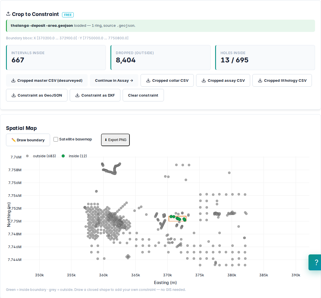
| Intervals inside | 667 of 9,071 |
| Intervals dropped | 8,404 |
| Holes inside | 13 of 695 |
Note: the map shows 12 collars inside the box, but 13 holes contribute intervals. Core crops on the desurveyed mid-point of each interval, not on the collar. One hole is collared outside the box and drills into it. A collar-based crop would lose those intervals.
Holes kept: TE-1, TE-2, TH1, TH2, TH3, TH4, TH5, TH6, TH31, TH35, TH37, TH39, TH40. All 13 (11 diamond, 2 percussion) have surveys, none is a duplicate collar, and the only overlaps among them were the two TH37 spot samples removed in §3. Export Cropped master CSV (desurveyed) for the next step.
5. Know the populations before deciding anything
Before going into Assay, statistics for these 667 samples are computed outside the app (plain Python, straight from the exported CSV):
| Zn (%) | |
|---|---|
| Mean | 2.245 |
| Median | 0.2 |
| Coefficient of variation (CV) | 2.66 |
| P95 / P99 / max. | 15.1 / 31.2 / 40.6 |
| Sample length median / mode | 0.7 m / 1.0 m |
The mean is eleven times the median, with a CV of 2.66. That shape can mean two things that call for very different treatments:
- one population with a few outliers → handled by top-cutting;
- a mixture of two populations (massive sulphide ore and wall rock) → handled by domaining.
A simple test tells them apart: look at where the metal sits.
| Samples with Zn ≥ | Share of total Zn metal |
|---|---|
| 0.5 % | 95.7 % |
| 1 % | 91.7 % |
| 2 % | 87.0 % |
| 5 % | 74.6 % |
Now split at 1 % Zn:
| n | Mean Zn | CV | |
|---|---|---|---|
| ≥ 1 % (inside the shell) | 170 | 8.26 % | 1.15 |
| < 1 % (outside) | 497 | 0.187 % | 1.26 |
The CV drops from 2.66 to 1.15 once the populations are separated. The high variability comes from mixing populations, not from outliers. That conclusion drives the next two decisions: do not cap high grades, and do separate domains.
6. Assay: choose the commodity, test the top-cut, build the domain
Upload the cropped master CSV to Orebit Assay. Assay recognises units from column names and converts zn_ppm, pb_ppm, cu_ppm to percent (÷ 10,000). The conversion is shown, not done silently.
Choose the primary commodity
By default Assay takes the first grade column, cu_pct, which is wrong for a zinc deposit. Choose zn_pct in the Commodity selector. The choice applies to validation, domaining, QAQC, the report and the PDF.
Top-cut: tested, then deliberately not applied
The Top-Cut tab looks for the disintegration point, where the upper tail of the distribution starts to break up. For Zn it is at 27.5 % (98.1st percentile).
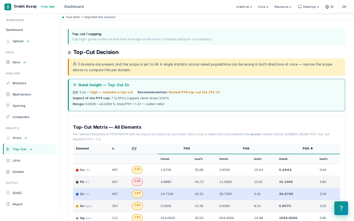
Decision: no top-cut on Zn. Reasons:
- §5 showed that the variability comes from mixed populations. Inside the mineralised domain the CV is only 1.15, well below the level at which geologists usually start considering a cap (about 1.5–2).
- 27–40 % Zn is sphalerite-rich massive sulphide, a real population, and exactly what was mined here. Capping it at 27.5 % removes real metal from the best ore.
- Top-cuts limit the influence of a few extreme samples on many blocks. The search strategy (§8) handles that better.
Deciding not to cap is as much a decision as capping, and it must be written in the report with its reasoning.
Domain: a 1 % Zn grade shell, because there is no lithology
Domain tab → method Grade shell (cut-off), cut-off 1 (% Zn).
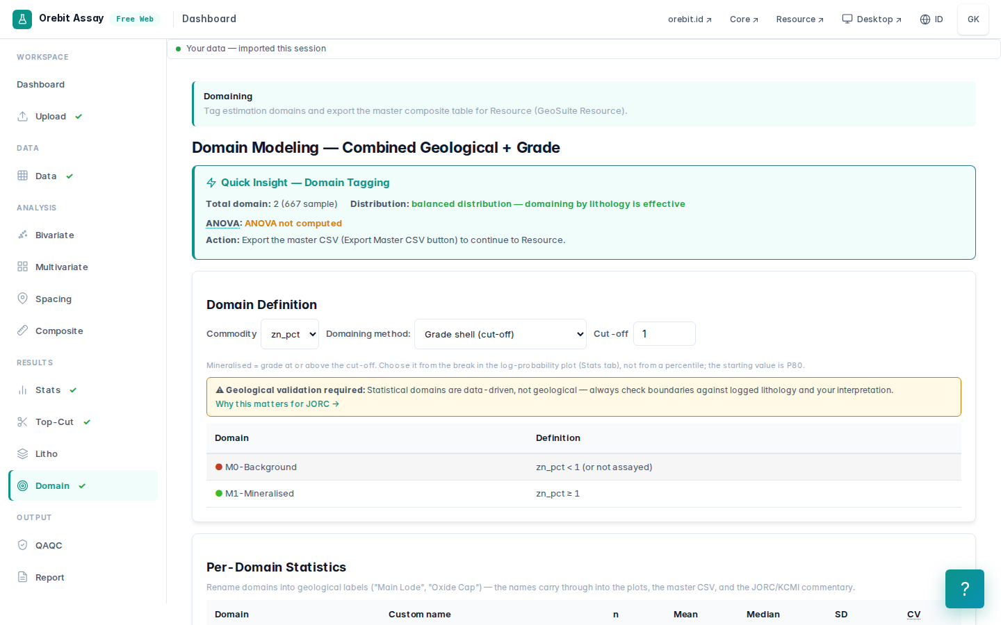
| Domain | Samples |
|---|---|
| M1-Mineralised (Zn ≥ 1 %) | 170 |
| M0-Background (Zn < 1 % or not assayed) | 497 |
Why 1 %: it captures 91.7 % of the metal (§5), separates the two populations with a reasonable CV, and is low enough not to "cut into" the ore. A domain cut-off is not an economic cut-off. It separates populations; it does not decide what is worth mining.
The limitation must be stated: a grade shell is not a geological domain. It is shaped by the grades themselves, so it tends to be optimistic at the edges (low samples between high ones are left out) and knows nothing about lithological contacts or structure. With lithology logging, the domains should come from massive sulphide / stringer / wall-rock contacts. That data does not exist here, so we use a grade shell and say so.
1 m compositing
Composite tab, length 1 m (the modal sample length).
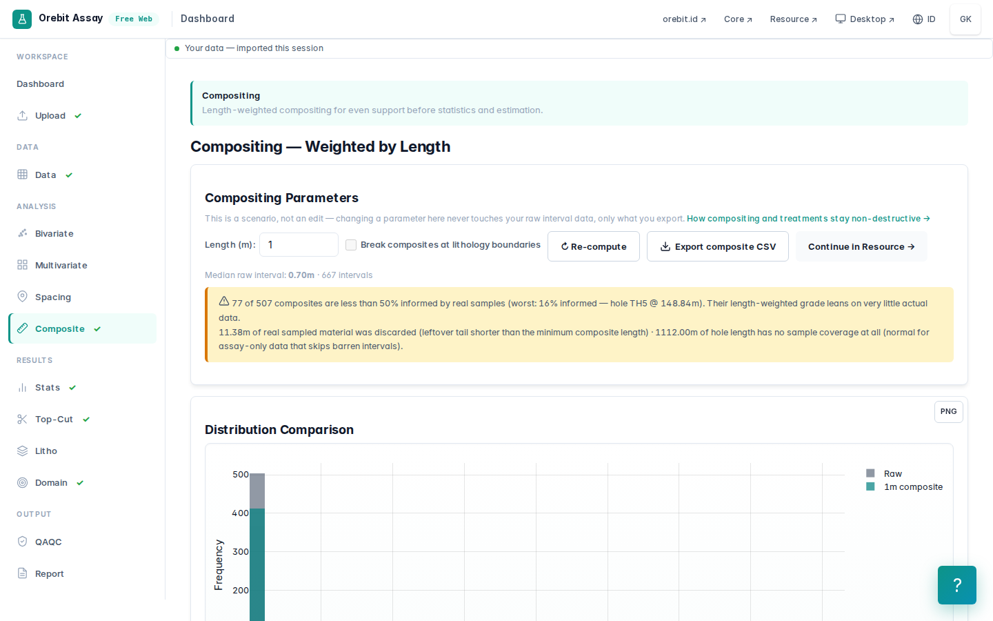
| Composites | 507 (M1: 98, M0: 409) |
| Real sampled length discarded (tails shorter than the minimum) | 11.38 m |
| Hole length with no samples at all | 1,112 m |
| Overlaps | 0 |
| Composites less than 50 % informed by real samples | 77 |
Core treats unsampled intervals as unknown, not zero. In compiled data, unassayed intervals are usually assumed barren by the driller, but that assumption is for the geologist to make, not the software. Every composite carries a coverage column. The yellow warning flags 77 composites that are less than half informed by real samples. Review them before estimating.
Export with Export composite CSV (exportMasterForEstimation). The file already carries coordinates, the domain, and grades in percent.
7. Resource: setup, variogram, block model
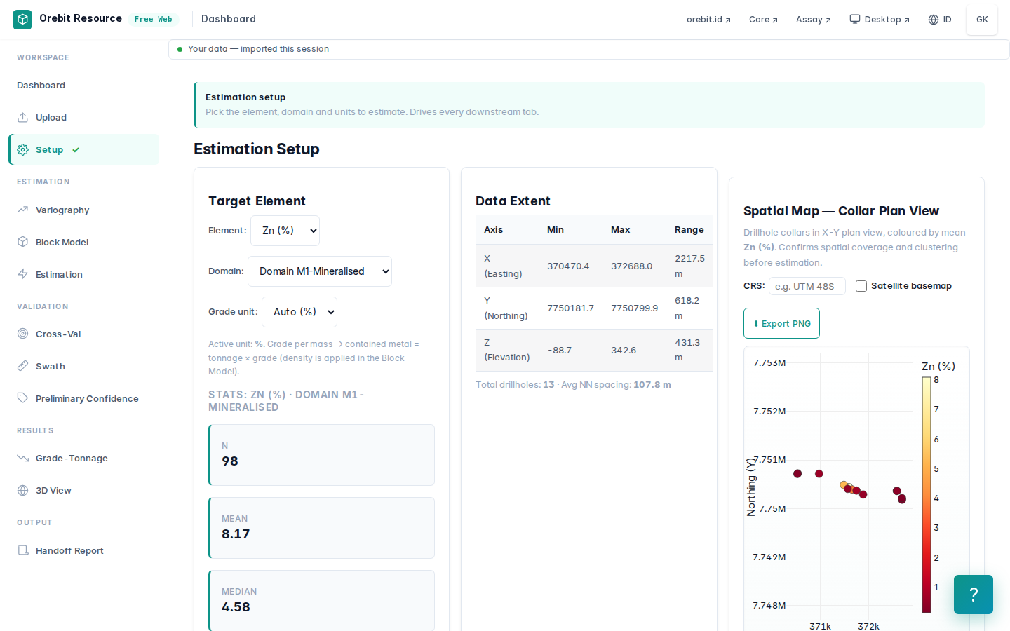
Upload the composites to Orebit Resource. On Setup choose element zn_pct and domain M1-Mineralised: 98 composites.
Variogram
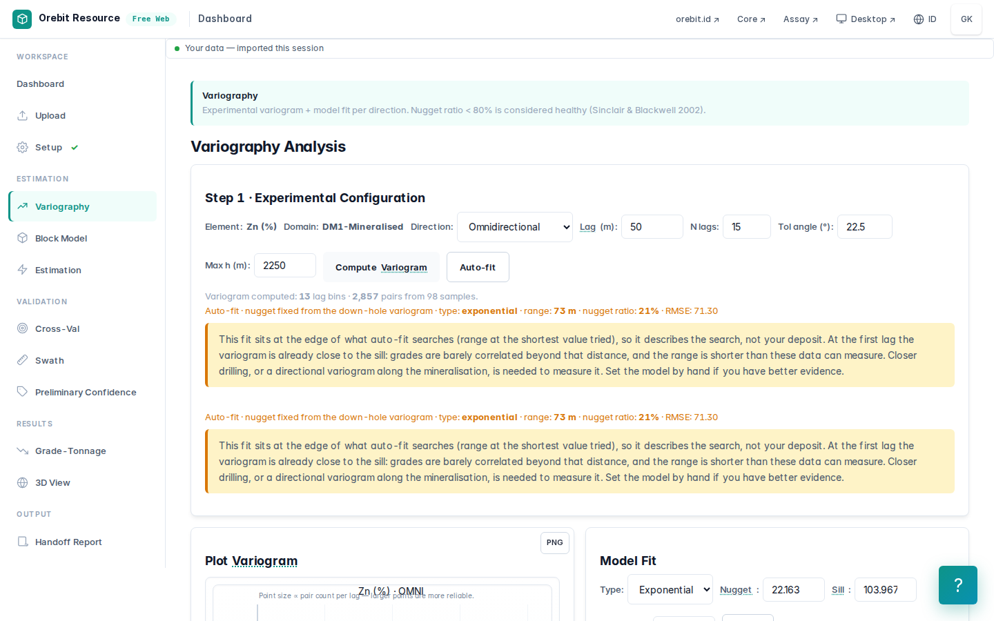
Down-hole first. Between holes the closest composites are about 90 m apart, so the nugget, the variability at zero distance, can only be read along the holes. Open Variogram Downhole on the Variography tab: pairs of samples within the same hole, 2 m lags. It finds 840 within-hole pairs, and γ rises from 22.2 (%²) at 1 m to 113.5 at 15 m. Real short-range structure: over a few metres the grade changes from massive sulphide to wall rock.
Then between holes. Compute the experimental variogram and Auto-fit. Because the down-hole variogram exists for this element and domain, auto-fit holds the nugget at the down-hole value and fits only the sill and range: exponential, nugget 22.2, sill 104.0 (%²), range 72.5 m. The nugget is about 21 % of the sill.
The app marks the range in yellow, and it should: 72.5 m is the shortest range the fit is allowed to try, not a measurement. The first lag says why. Over 0–50 m, where almost every pair is a down-hole pair, γ is already 77.4, 97 % of the data variance (80.0), and the down-hole variogram passes the variance by 15 m. Down the hole, Zn grade stops being correlated within about 10–15 m, roughly the thickness of a lens. Along strike the continuity is not measured at all: the closest holes are 90 m apart.
What that means for the estimate: with holes about 90 m apart (below), a block between holes gets close to the local mean of its neighbours. That smoothing is forced by the drill spacing, not by a modelling choice. Only infill drilling can resolve it, and a Competent Person will weigh it in any classification.
A correction this vignette forced. Earlier revisions reported nugget 67.2, "60 % of the sill". That was the ceiling of the fitting grid (the nugget search stopped at 60 %), reported as if it were a property of the deposit. The same artefact appeared on Babbitt and on an epithermal gold dataset. The grid now reaches 90 %, the nugget comes from the down-hole variogram, and a fit that lands on an edge of the grid is flagged. Cross-validation improved with it (OK slope 0.68 → 0.75, §9).
Block size
The app suggests 15 × 15 × 8 m. The Estimation tab reports nearest between-hole spacing: median 91 m, P90 96 m. Blocks much smaller than about a quarter of the drill spacing only create an illusion of resolution: kriging 15 m blocks between holes 90 m apart produces hundreds of nearly identical blocks that look like detail and are not.
Used: 25 × 25 × 10 m (about ¼ of the hole spacing; 10 m is a typical bench/level height). Result: 20,967 blocks (84 × 20 × 29). Density is left at the default 2.8 t/m³, which the app correctly flags as ASSUMED (§11).
8. Estimation: the most important lesson in this vignette
Three runs on the Estimation tab, with the same composites and the same variogram. Only two decisions change: the domain boundary and the search strategy.
Run A — default parameters, no domain boundary
Switch Keep blocks inside the domain off. That is how every GeoSuite version before 25 September 2026 behaved. Use the auto-suggested search (1.5 × the variogram range, widened for sparse data): 218 × 218 × 135 m, minimum 2 composites.
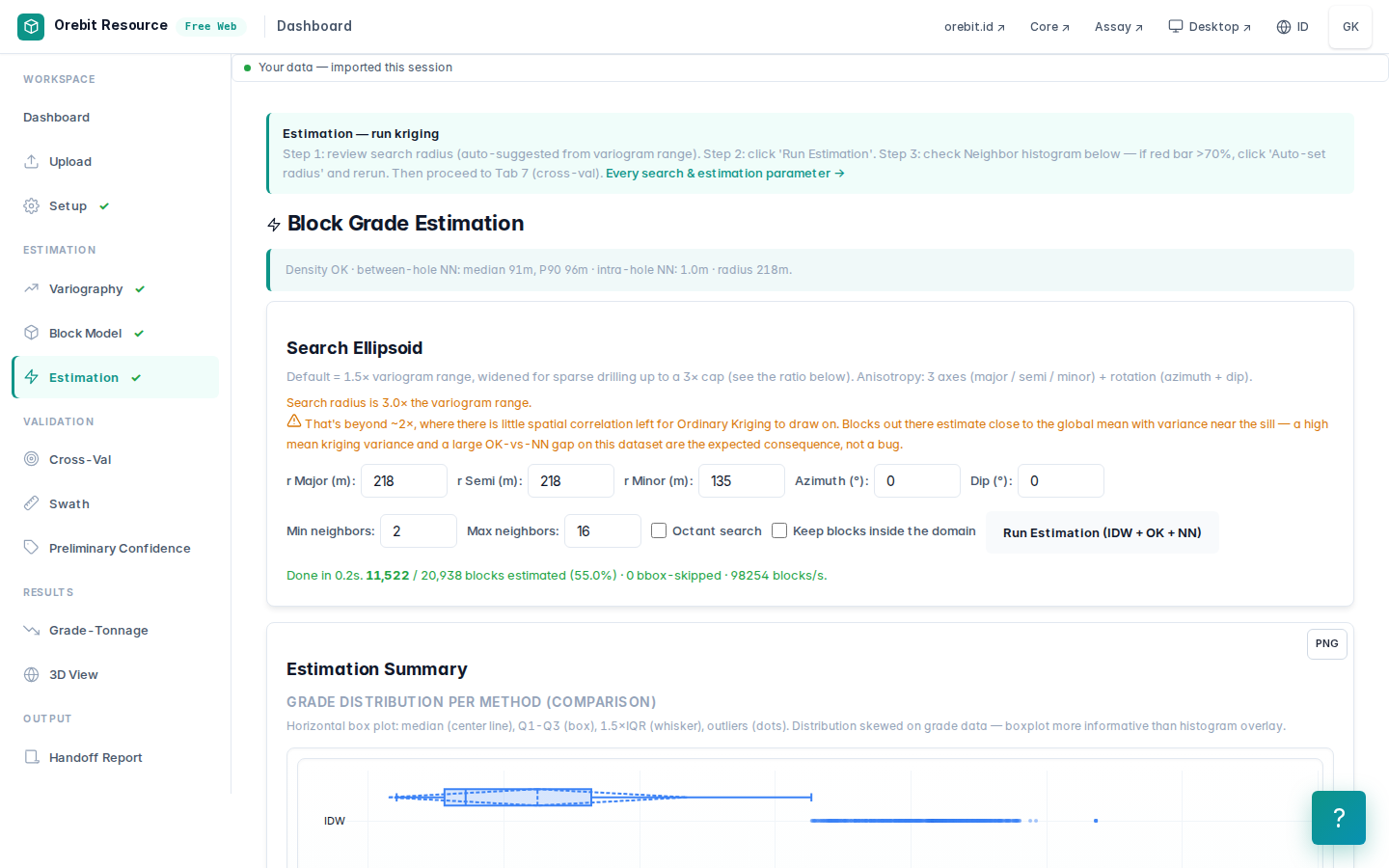
| Blocks estimated | 11,522 of 20,967 |
| Tonnes (2.8 t/m³) | 202 Mt |
| Zn metal | 11.9 Mt |
| Lowest OK grade | 1.05 % |
That is 43 times historical production. No error, no red warning, and completely wrong. The estimate uses only M1 composites (all ≥ 1 % Zn) and spreads that grade into every block within 218 m, including hundreds of metres of wall rock. The lowest block grade is 1.05 % because no low sample ever takes part.
A domain boundary without a wireframe
No lithology means no wireframe. But the 409 M0 composites (Zn < 1 %) still know where the ore is not. GeoSuite now uses all of them as the boundary: a block belongs to domain M1 only if its nearest composite, of any domain and measured with the same search ellipsoid, is an M1 composite. This is nearest-neighbour domain assignment, the standard way to build a hard boundary from drilling when no geological model exists yet. It is on by default.
This feature was added to GeoSuite because of Run A in this vignette.
Run A2 — default parameters, with the domain boundary
| Blocks estimated | 810 |
| Blocks within reach removed by the domain boundary | 20,123 |
| Tonnes | 14.2 Mt @ 7.38 % Zn |
The boundary alone cuts the tonnage 14-fold. But 14 Mt is still 3 times production, because the round 218 m ellipsoid still reaches far into undrilled ground. At the edge of the drilling there are no M0 composites to "reject" a block, so the outermost M1 composite becomes the nearest one for blocks hundreds of metres away.
Run B — domain boundary + a geologically constrained search
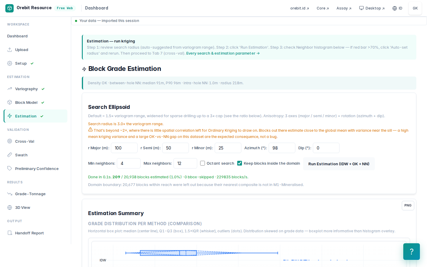
Strike from the composite distribution (PCA): azimuth 98°, roughly east–west, matching the TH-series hole distribution. Parameters:
| Reason | ||
|---|---|---|
| r Major | 100 m | about half the along-strike hole spacing |
| r Semi | 50 m | the across-strike geometry is unresolved (below) |
| r Minor | 25 m | lens thickness is far below 100 m |
| Azimuth / dip | 98° / 0° | strike from the data; dip cannot be determined reliably |
| Min / max composites | 4 / 12 | no block is informed by a single intercept |
| OK | IDW | NN | |
|---|---|---|---|
| Blocks | 209 | 209 | 209 |
| Mean Zn grade | 8.09 % | 8.72 % | 9.24 % |
| Tonnes | 3.658 Mt | ||
| Zn metal | 295.8 kt |
The dip of the lens is unresolved. Cross-sections between holes give dips of 2°, 12° and 41°, which are inconsistent. With 13 holes and no lithology, the lens orientation cannot be determined, so the ellipsoid is kept flat and tight across strike. That is a conservative choice, and it is also this result's biggest limitation.
Global mean check: the NN mean (9.24 %) is 14 % above OK (8.09 %). Practice looks for agreement within ±5 %. With only 209 blocks, the NN mean is dominated by a few high-grade composites that happen to be nearest to many blocks, while OK smooths them. This yellow flag points the unusual way: OK is conservative relative to the nearest data. A better reference is the declustered composite mean (Declustering in Assay).
9. Cross-validation
Cross-Val tab (leave-one-out, n = 92 composites):
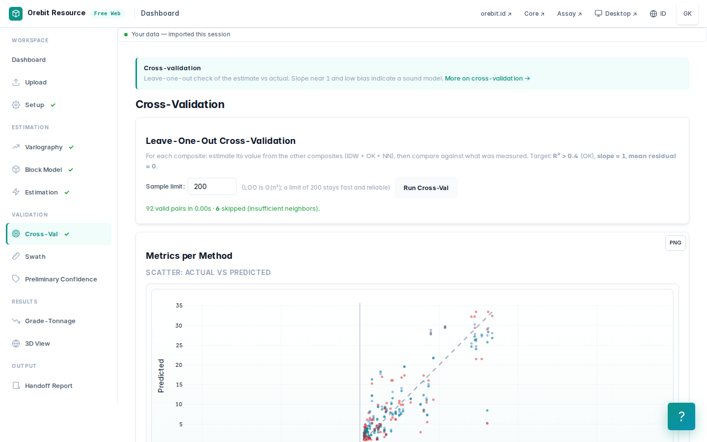
| OK | IDW | NN | |
|---|---|---|---|
| Regression slope (estimate on actual) | 0.75 | 0.77 | 0.82 |
| r² | 0.75 | 0.75 | 0.71 |
| Mean bias (estimate − actual) | +0.08 | +0.24 | +0.19 |
| RMSE | 4.60 | 4.62 | 5.07 |
How to read it: OK is globally unbiased (+0.08 % Zn on a mean of 8.43 %) but conditionally biased. A slope of 0.75 means high grades are under-estimated and low grades over-estimated. That is the smoothing you expect when the correlation range is shorter than the hole spacing (§7). It means the grade-tonnage curve at high cut-offs must be read with care: tonnes above a high cut-off tend to be too many at too low a grade. A slope of 0.8–0.9 or better is usually sought for an estimate used for block-by-block decisions.
10. Confidence screen and grade-tonnage
Confidence screen
The Preliminary Confidence tab splits the 209 blocks by distance to data and number of holes:
| Tier | Blocks |
|---|---|
| High confidence | 39 |
| Medium confidence | 72 |
| Low confidence | 98 |
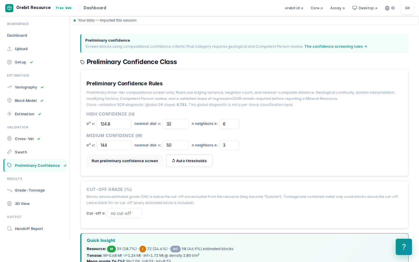
This is a computational screen, not a Measured / Indicated / Inferred classification. KCMI 2017 and JORC 2012 set no numeric thresholds. Classification is a Competent Person's written judgement, weighing geology, QAQC, density and continuity. That is why GeoSuite deliberately does not use those terms.
One thing worth noting: the mean grade of the high + medium blocks (7.70 %) is lower than that of all blocks (8.09 %). The highest grades sit in the blocks furthest from data, the classic signature of extrapolation. That is one more reason to distrust the high-cut-off numbers.
Grade-tonnage, checked independently
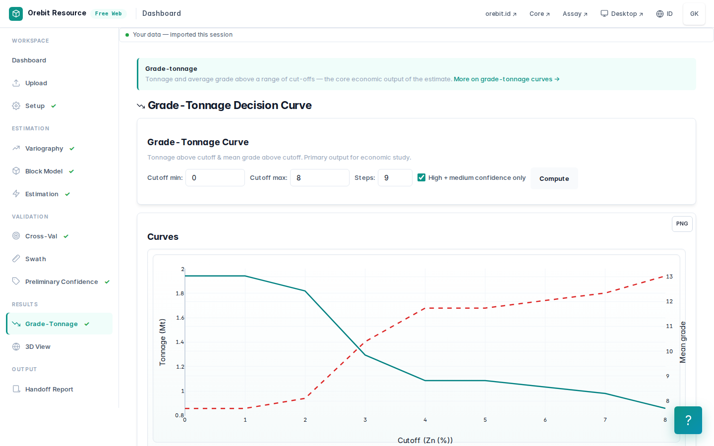
The curve on the Grade-Tonnage tab is computed by the app. The table below is recomputed independently from the exported block model (exportBlockCSV) in plain Python and compared with the app's curve. test_vignettes.py fails the build if they disagree.
| Zn cut-off | Tonnes (Mt) | Zn grade | Zn metal (kt) | High + medium only: Mt @ % |
|---|---|---|---|---|
| 0 / 1 % | 3.658 | 8.09 % | 295.8 | 1.943 @ 7.70 |
| 2 % | 3.465 | 8.44 % | 292.6 | 1.820 @ 8.10 |
| 3 % | 2.590 | 10.47 % | 271.1 | 1.295 @ 10.38 |
| 5 % | 2.188 | 11.76 % | 257.2 | 1.085 @ 11.73 |
| 8 % | 1.768 | 13.00 % | 229.9 | 0.858 @ 13.02 |
11. Density: one number that moves tonnage by ±30 %
The KCMI tab shows the density basis as:
ASSUMED uniform default — not measured. Enter the deposit's measured SG before reporting tonnage.
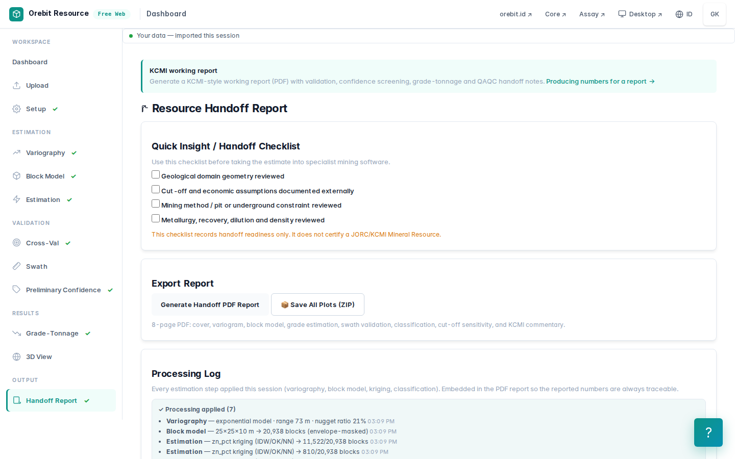
Massive sulphide ore with sphalerite, galena and pyrite typically runs 3.2–4.0 t/m³, not 2.8. Tonnage scales directly with density, so 2.8 may under-state massive-sulphide tonnage by up to about 30 %, while 2.8 may be fine in stringer / disseminated zones. Density must be measured, per domain or regressed against Fe+S+Zn+Pb. Until then the tonnage is not reportable.
For scale: the same 209 blocks at 3.6 t/m³ give 4.702 Mt, not 3.658 Mt.
12. Sanity check against historical production
| Tonnes | Zn | |
|---|---|---|
| Production 1989–1998 | 4.7 Mt | 8.3 % |
| Run A: no domain boundary | 202 Mt | 5.88 % |
| Run A2: domain boundary, default search | 14.2 Mt | 7.38 % |
| Run B: boundary + geological search (2.8 t/m³) | 3.7 Mt | 8.09 % |
| Run B at a massive-sulphide density of 3.6 t/m³ | 4.7 Mt | 8.09 % |
| Run B, high + medium confidence only | 1.9 Mt | 7.70 % |
The grade is within about 3 % of the mined grade. The tonnage is 78 % of production at the assumed density, and practically the same at a reasonable massive-sulphide density.
Do not celebrate too early. Part of this agreement is coincidence, and a senior geologist has to say so:
- Production is not a resource. The mine extracted part of the deposit at an economic cut-off with dilution (which lowers the grade), then closed for economic reasons. The deposit was later redeveloped, so mineralisation remained after 1998.
- Unresolved orientation. A horizontal ellipsoid on a lens of unknown dip can put volume in the wrong place even when the total happens to come out close.
- The domain boundary rests on one cut-off (1 % Zn). Move it to 0.5 % or 2 % and the tonnage moves. Without a lithology wireframe, this volume still depends on that decision.
The honest conclusion: with a domain boundary and a geologically constrained search, 13 holes with no lithology produce a plausible order of magnitude, grade and tonnage against the mine's history. But the volume and its classification are still not reportable. That is what a screen is for: telling you what to do next, not replacing it.
13. This is not a Mineral Resource. What it would take:
- [ ] Lithology logging and a 3D geological model of massive sulphide / stringer / wall rock, replacing the grade shell;
- [ ] A resolved lens orientation (interpreted sections, structural data, or more drilling);
- [ ] Measured density per domain;
- [ ] QAQC: standards (CRMs), blanks and duplicates for the campaigns used, lab certificates, including resolving TH35's Au 1,380 g/t;
- [ ] Collar and downhole survey verification (coordinate system, survey method);
- [ ] A geologist's decision on unsampled intervals;
- [ ] Swath-plot validation, and reconciliation against historical production and existing mine voids;
- [ ] Classification and reporting by a Competent Person under KCMI 2017 / JORC 2012.
Try it yourself
- Change the domain cut-off to 0.5 % and 2 %. Watch how much metal enters or leaves the domain, and how the in-domain CV changes.
- Switch Keep blocks inside the domain off for Run B. How many tonnes are added, and where do the extra blocks sit?
- Re-run Run B with minimum 2 composites and octant search on. Which blocks change most?
- Raise r Semi to 100 m and look at the cross-validation and the OK/NN ratio.
Reproducing this vignette
node build/build.mjs                                     # build Core/Assay/Resource into dist/
python3 docs/vignettes/tools/run_thalanga.py             # ~90 s; writes data/thalanga.json + img/
python3 docs/vignettes/tools/run_thalanga.py --no-shots  # skip screenshots
The script drives the same app build users get, in Chromium, step by step as above. The key numbers are re-derived independently from the exported files.
Attribution
Data: © State of Queensland (Geological Survey of Queensland), NEQ Deposit Atlas – Thalanga (ds100103), licensed under CC BY 4.0. Loaded as published. The only changes are the two deletions and one blanked value described in §3, all recorded in the CHANGE_LOG. The area boundary (thalanga-deposit-area.geojson) was made for this vignette. Historical production: mining-technology.com, Thalanga Zinc Project, Queensland.
Source of this page: docs/vignettes/en/01-thalanga-vms.md · GPL-3.0 · github.com/ghoziankarami/geosuite